... from an idea to superior design performance with mathematical modelling and engineering analysis ...
Turbulent flow separation and reattachment
Introduction
Flow separation occurs in many aerodynamic flows of interest: airfoils,
road vehicles, HVAC equipment, and in built environment. It leads to loss
of lift, increase of drag, and in general causes pressure losses that cannot
be recovered. The backward facing step geometry offers one of the simplest
geometrical arrangements to study the separation and reattachment process [1].
For that reason, the flow over a backward facing step has become a very popular CFD
benchmark case with available experimental data [1-3] and the Direct Numerical
Simulations (DNS) results [4]. Due to sensitivity of the separation and reattachment
process to the turbulence behaviour and the pressure distribution, the case
is widely used for validation of turbulence models [5].
Objectives
CFD simulations shall be conducted for the flow over a backward facing step
with 0° and 6° expansion angle of the downstream section
in order to assess the performance of the applied turbulence models.
The CFD simulation results shall be used to calculate the vertical distribution of the flow velocity,
streamwise variation of the wall friction and pressure coefficients, and the reattachment location
in order to compare them with the experimental data [1].
The validation case tests not only the ability of the turbulence model to predict recirculation
and reattachment, but also appropriateness and sensitivity of the imposed boundary
(inlet and wall) conditions. Larger deviations are expected when the expansion angle imposes
an adverse pressure gradient.
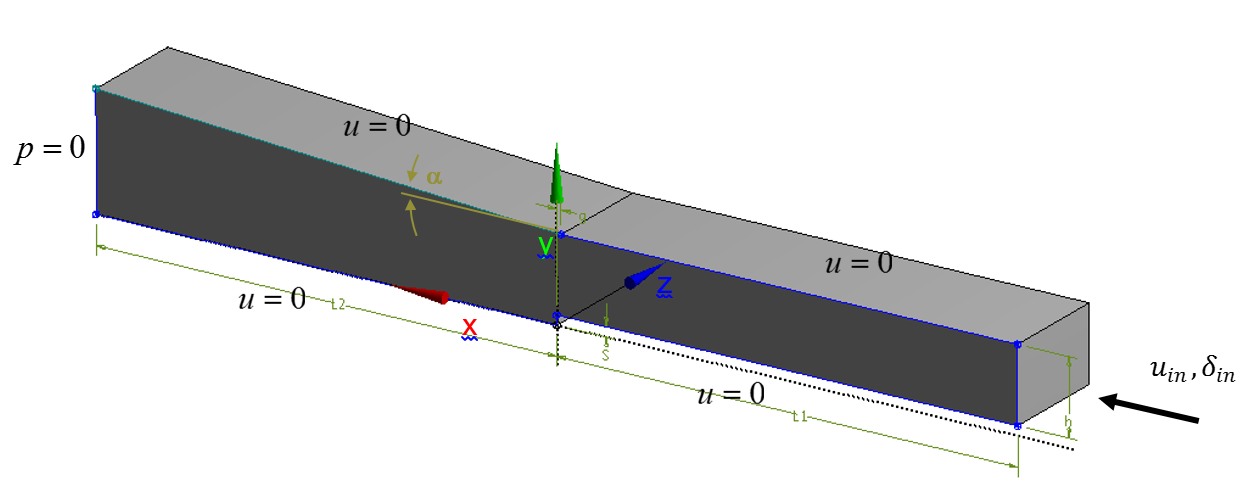
Geometry
Step height (S) is 12.7 mm.
Height of the upstream section (h) is 8 S.
Length of the upstream section (L1) is 50 S.
Length of the downstream section (L2) is 50 S.
Flap angle (`alpha`) is 0 and 6°.
Flap hinge is offset from the step upstream by 6 mm.
Width in z-direction is 12 S (although the flow conditions are statistically 2D).
The length of the upstream section (L1) can be modified as long as the boundary layer thickness and
the inflow profiles are adjusted appropriately.
Loading
The mean flow velocity profile is prescribed at the inlet:
`u_(\i\n)=u_(ref) (y/delta_(\i\n) )^(1//7)` for `y < delta_(\i\n)`
where `u_(ref)` is the far-field velocity and `delta_(\i\n)` is the boundary layer thickness
at the inlet location.
The profile needs to be consistent with the experimentally reported boundary layer thickness
along the lower wall [1]: `delta_4=0.019` `"m"` at `x_4=`-`4S`.
The friction force and its variation along channel walls further develop the flow profile,
and influence its separation and reattachment.
The expanding angle (`alpha`) of the channel downstream section imposes a positive pressure gradient
that reduces the overall flow velocity and increases turbulence production.
Material properties
Material properties of incompressible air:
`nu` is kinematic viscosity of 0.000015 m2/s [1];
`rho` is density of 1.204 kg/m3.
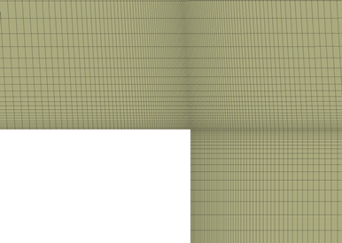
Meshing
In all simulated cases, the numerical grid consists of hexahedral grid elements
elongated in the streamwise direction, and refined near the wall (i.e. bottom, top and the step).
The grid spacing is refined in the x-direction from 5.3 mm near the inlet and the outlet to
0.01 mm near the step. In the y-direction, the largest grid spacing (1.5 mm) that is in the centre of the channel
is reduced to 0.01 mm near both horizontal walls.
In the z-direction, the 2D grid elements are extruded for a single grid spacing
across the simulation domain.
Section of the hexahedral numerical grid refined near the step and the flap
Initial conditions
Steady-state problem, initial conditions can be arbitrary.
Boundary conditions
At the inlet, mean flow velocity profile and turbulent model variables are prescribed:
`u_(\i\n) = u_(ref)(y/delta_(\i\n))^(1//7)`
`k_(\i\n) = max|k_(ref),(u_(tau)^2)/(C_mu^(1//2))(1-y/delta_(\i\n))|` and
`epsilon_(\i\n) = C_mu^(3//4)(k_(\i\n)^(3//2)/(kappa y))`
where
`C_mu = 0.09` is a turbulence model constant;
`kappa = 0.41` is the von Karman constant;
`u_(ref) = 44.2` `"m"//"s"` is the far-field velocity [1];
`k_(ref) = 0.0004` `u_(ref)^2` is the far-field turbulence kinetic energy;
`delta_(\i\n)` is the boundary layer thickness at the inlet that is related to the boundary layer thickness at `x_4`:
`delta_(\i\n)^(5//4) = delta_4^(5//4)-0.2931(x_4-x_(\i\n))(u_(ref)/nu)^(-1/4)`
`u_(tau)` is the shear velocity that is defined as
`(u_(tau)/u_(ref))^2 = 0.0228((u_(ref\ ) delta_(\i\n))/nu)^(-1//4)`
The no-slip boundary condition `u=0.0` `"m"//"s"` is assigned to the bottom and the top wall.
For the outlet boundary, fixed relative pressure (e.g. `p = 0.0` `"Pa"`) is appropriate. The pressure
absolute value does not influence the flow velocity results.
For the vertical X-Y surfaces, the symmetry or equivalent conditions shall be used.
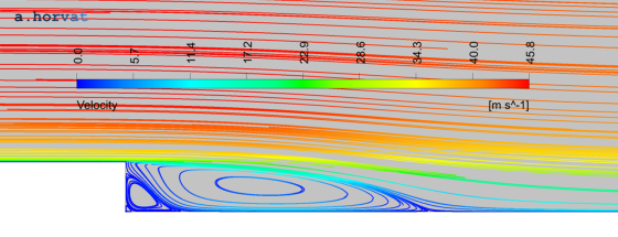
Results
Steady-state simulations were performed using the Shear Stress Transport (SST) turbulence model
in a double precision CFD solver.
Flow velocity streamlines in the channel for the 0° flap angle
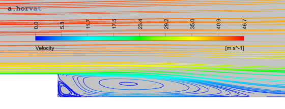
Flow velocity streamlines in the channel for the 6° flap angle
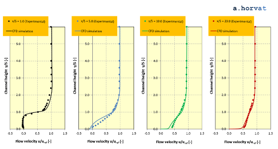
The cross-channel profile of mean streamwise velocity (`u`) is extracted from
the CFD simulation results and compared with the experimental data [1, 2 & 5].
The diagrams below present two sets of such data for the 0 and 6° flap angle,
respectively. The coordinate `x` represents the downstream distance from the step location
normalised with the step height (`S`).
Comparison of flow velocity profiles (`u//u_(ref)`) for the 0° flap angle at x/S = 1.0, 5.0, 10.0 and 20.0
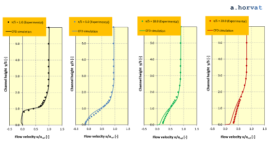
Comparison of flow velocity profiles (`u//u_(ref)`) for the 6° flap angle at x/S = 1.0, 5.0, 10.0 and 20.0
For validation purposes, quadratic mean (or RMS) of deviation between the experimental data and
the CFD simulation results is calculated for the flow velocity profiles (`u//u_(ref)`) and 0° flap angle:
Location x/S
RMS of deviation
1.0
0.051
5.0
0.058
10.0
0.053
20.0
0.041
and for the 6° flap angle:
Location x/S
RMS of deviation
1.0
0.046
5.0
0.053
10.0
0.059
20.0
0.075
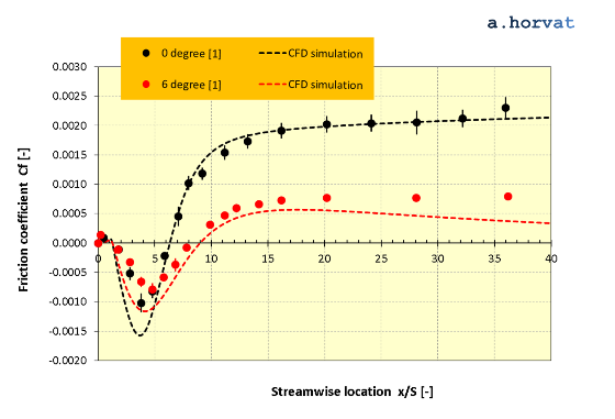
Wall friction coefficient is defined as
`C_f = 2 (tau_w)/(rho u_(ref)^2)` where `tau_w = mu del_y u |_(y=0)` is the shear stress at the wall,
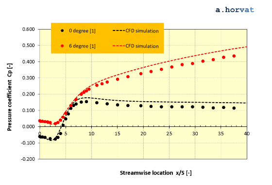
and the pressure coefficient as
`C_p = 2 (p-p_(ref))/(rho u_(ref)^2)` where `p_(ref)` is the far-field static pressure at `x=`-`4S`.
Their values are calculated for the bottom wall of the simulation domain and compared with
the experimental data [1].
Wall friction coefficient `C_f` along the bottom wall
Pressure coefficient `C_p` along the bottom wall
Quadratic mean (or RMS) of deviation between the experimental data and the CFD simulation results
is presented below for the friction coefficient (`C_f`):
RMS of deviation
0° flap angle
0.0002758
6° flap angle
0.0002815
and for the pressure coefficient (`C_p`):
RMS of deviation
0° flap angle
0.02386
6° flap angle
0.02634
The location of the vortex reattachment is identified by the flow reversal and therefore
by the change in the wall friction coefficient:
`C_f < 0 -> C_f > 0`.
The reattachment length (`x_r`), which is the distance from the step to the location of the flow
direction reversal, is calculated and compared to the experimental data [1 & 2]:
Experimental data [1 & 2]
CFD results
0° flap angle
`x_r//S = 6.26 +- 0.10`
`x_r//S = 6.33`
6° flap angle
`x_r//S = 8.30 +- 0.15`
`x_r//S = 9.00`
Note that the reattachment length (`x_r`) is normalised with the step height (`S`).
D. M. Driver and H. L. Seegmiller, Features of reattaching turbulent shear layer in divergent channel flow, AIAA Journal, Vol. 23, No. 2, Feb. 1985, pp. 163-171.
S. D. Hall, M. Behnia, G. Morrison and C. A. J. Fletcher, Comparison of measurement techniques for a turbulent two phase backward facing step flow, ASME Heat and Mass Transfer Conference, Hawaii 1999.
S. Patil and D. Tafti, Wall modeled large eddy simulation of flow over a backward facing step with synthetic inlet turbulence, 49th AIAA Aerospace Sciences Meeting including the New Horizons Forum and Aerospace Exposition, 4 - 7 January 2011, Orlando, Florida.
J. -Y. Kim, A. J. Ghajar, C. Tang and G. L. Foutch, Comparison of near-wall treatment methods for high Reynolds number backward-facing step flow, Int. J. Comp. Fluid Dynamics, Vol. 19, No. 7, October 2005, pp. 493-500.
Dr Andrei Horvat
M.Sc. Mechanical Eng.
Ph.D. Nuclear Eng.