... from an idea to superior design performance with mathematical modelling and engineering analysis ...
Oscillatory motion of viscous boundary layer
Introduction
The Stoke's oscillating plate case is one of transient flow examples that
offers a closed-form solution. The fluid motion, which is stimulated by
an oscillating boundary, is dominated by viscous forces. It can be shown
that the system of transport equations is reduced to a diffusion equation
for a single velocity component [1, 2].
The integration of the diffusion equation over a longer time interval shall
expose numerical diffusion of the applied spatial and temporal discretisation.
Objectives
Examine the accuracy of transient solver and the extent of false, numerical
diffusion by comparing the velocity distribution with the analytical solution
throughout the simulation time interval. The numerical error is manifested
by the accelerated velocity decay and the phase shift of the oscillatory motion.
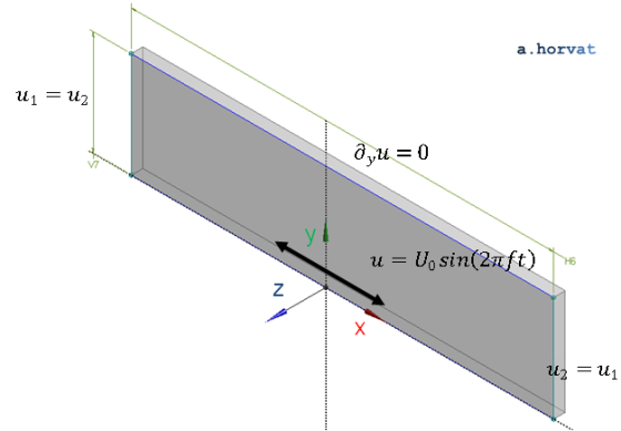
Geometry
Length of the simulation domain (H6) is 8.0 m.
Domain height (V7) is 5.0 m.
Domain width is 0.2 m (although not important due to the case two-dimensionality).
Loading
Sinusoidal oscillations in the x-direction are forced by prescribing a plate velocity
function `u=U_0 sin(2 pi f t)` to the bottom surface where:
`U_0` is the velocity amplitude set to 1.0 m/s;
`f` is the forced oscillation frequency set to 1.0 Hz;
`t` is time.
Material properties
Propagation of the low speed oscillatory motion depends solely on the kinematic viscosity
of the fluid:
`nu` is kinematic viscosity of 1.0 m2/s (comparable to glycerol)
Meshing
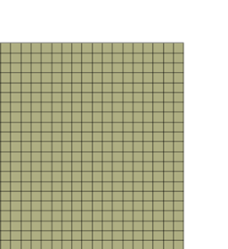
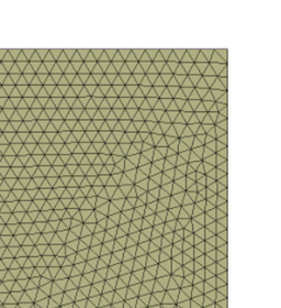
Influence of two different types of grid elements is investigated. The first simulation
is performed using the grid with tetrahedral elements and the second with the hexahedral
elements. a)
b)
Section of the numerical grid: (a) hexahedral and (b) tetrahedral elements
For both cases, the size of elements is set to 0.1 m and kept uniform across the entire simulation domain.
In the z-direction, the 2D grid elements are extruded for a single grid spacing across the
simulation domain.
Initial conditions
Zero velocity (`u`) and relative pressure (`p_(rel)`) for the whole domain
Boundary conditions
The bottom plate has a prescribed velocity `u=U_0 sin(2 pi f t)` with no slip
boundary conditions.
At the top surface, slip boundary conditions shall be used.
The vertical Y-Z surfaces at `x=x_(min)` and `x_(max)` have periodic boundary conditions
for the streamwise velocity (`u_1=u_2`) assigned to them.
For the vertical X-Y surfaces, the symmetry or equivalent conditions shall be used.
Results
The analytical solution is `u=U_0 e^(-kz) sin(2 pi f t - k z)` where:
`k = sqrt( pi f//nu)` is the wave number;
`nu` is fluid kinematic viscosity.
Induced flow velocity (red) and particle displacement (black)
The simulation results were obtained with the timestep of `1//32f` using a single precision CFD
solver.
The calculated velocity distribution are compared to the analytical solution at different
heights (`y`) in the simulation domain. The following elevations are advised: `y=0.1`, `0.2`, `0.4`, `0.8` and `2.0` `"m"`.
Time variation of the velocity (`u`) at `y =0.1` `"m"`
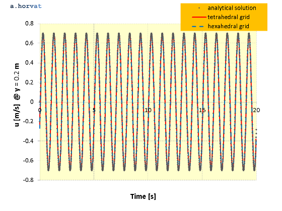
Time variation of the velocity (`u`) at `y =0.2` `"m"`
Time variation of the velocity (`u`) at `y =0.4` `"m"`
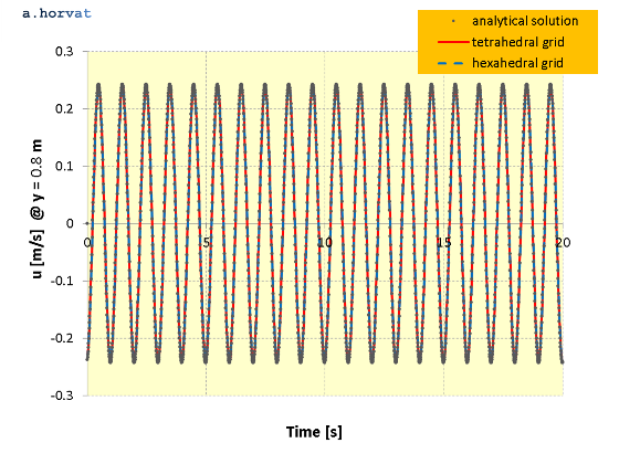
Time variation of the velocity (`u`) at `y =0.8` `"m"`
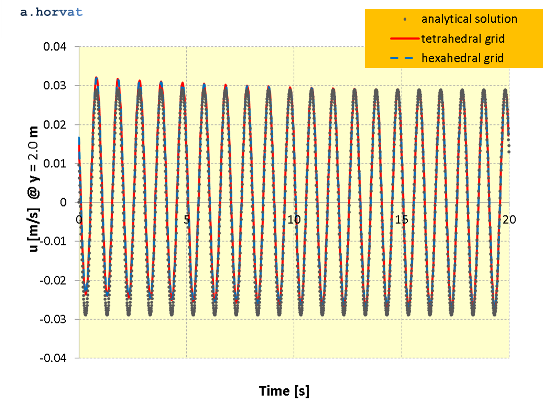
Time variation of the velocity (`u`) at `y =2.0` `"m"`
Dissipation of the velocity amplitude relative to the analytical solution (`u"/"u_a-1`)
as well as its phase shift (`Delta t`) are calculated. Smaller are the velocity amplitude difference
and the phase shift, lower is the false, numerical diffusion.
When using the tetrahedral numerical grid, the CFD simulation yields a reduced velocity
amplitude (`u`) in comparison to the analytic solution (`u_a`):
0.07% at y = 0.1 m;
0.14% at y = 0.2 m;
0.43% at y = 0.4 m;
1.42% at y = 0.8 m;
3.17% at y = 2.0 m.
Similarly, when using the hexahedral mesh, the following reduction of the velocity
amplitude (`u`) in comparison to the analytic solution (`u_a`) is observed:
0.47% at y = 0.1 m;
0.36% at y = 0.2 m;
0.50% at y = 0.4 m;
1.79% at y = 0.8 m;
3.74% at y = 2.0 m.
The velocity amplitudes that are used in the calculation were recorded 60 periods from the
start of the simulation.
No time delay between the calculated velocities and the analytical solution
was detected. It is believed that the time delay is smaller than the integration timestep used
in the CFD simulations.
 a)
a)
 b)
b)