... from an idea to superior design performance with mathematical modelling and engineering analysis ...
Poiseuille flow near the wall
Introduction
Most of flow scenarios can be categorised as wall-bounded flows, where momentum,
heat and/or mass is transferred between the solid structure and the bulk of
the flow. Wall effects are responsible for generation of a boundary layer,
introduction of vorticity, fluctuations and ultimately turbulence to the
fluid flow. For that reason, the approximation accuracy of the flow near-wall
effects is of extreme importance in Computational Fluid Dynamics (CFD).
In the turbulent flow regime, the transfer between the wall and the flow is
characterised by a thin viscosity dominated sublayer. Its correct approximation
is challenging for most of the turbulence models, which have been developed and
tuned for free stream decaying turbulence. Channel flow is one of wall-bounded
flow scenarios, which has been extensively studied [1-4].
Objectives
Accurate approximation of the velocity and the temperature profile in turbulent
channel flow requires a specially adopted turbulence model (e.g. low-Reynolds
number turbulence model) where Reynolds (or subgrid) stresses and the related
eddy viscosity are suppressed in the viscosity dominated near wall region.
The validation case tests the ability of the implemented turbulence model to
predict flow conditions in a highly anisotropic environment where the near-wall
effects are prevalent. Comparing the calculated velocity and temperature with
the results from Direct Numerical Simulations (DNS) [1-3] shall expose any
modelling deficiency and/or numerical errors (e.g. discretisation mistake, false
numerical diffusion, equation under-relaxation).
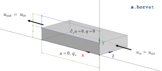
Geometry
Height of the half-channel (H1 = H2) is `delta`.
Length of the simulation domain (L) is 6.4 `delta`.
Width in z-direction is 3.2 `delta`.
The validation case is fully parametric and therefore the value of `delta` can be arbitrary.
Selective testing was performed with `delta` = 0.1 m.
The simulation domain can cover only half of the channel due to symmetry of the time
averaged flow field across the channel horizontal (X-Z) mid-plane. The channel width can be also reduced as the time averaged flow conditions are two-dimensional.
Loading
The periodic flow in the channel is induced with a source term in the x-component of the momentum transport equation:
`S_M = -(dp)/(dx) = tau_w/delta = (rho u_tau^2)/delta = rho/delta((Re_tau mu)/(rho delta))^2`
where
`Re_tau` is friction (or shear) Reynolds number
`mu` is dynamic viscosity
`rho` is fluid density
`delta` is the channel half-width
Two cases with different Reynolds numbers are considered: `Re_tau = 180` (for `Pr = 0.71` & `5.0`)
and `Re_tau = 395` (for `Pr = 0.71`).
If heat flux (`q_w`) is imposed at the horizontal wall, the enthalpy increases linearly through the simulation domain,
and therefore:
`(d(:T_m:))/(dx)=q_w/(rho c_p (:u:) delta)`
where
`u` is the flow velocity in x-direction
`(:u:)` is the channel average u velocity
`(:T_m:)=(:uT:)//(:u:)` is the mass flow averaged temperature
The temperature field can be then linearised
`-T + (d(:T_m:))/(dx) = theta`
by using the source term in the energy transport equation:
`S_E = u q_w/((:u:) delta)`
The exact value of the imposed wall heat flux (`q_w`) is not important in the parameterised system. Selective testing
has been performed with `q_w = 10` `"W"//"m"^2` (for `Pr = 0.71`), and `200` `"W"//"m"^2` (for `Pr = 5.0`).
Material properties
Two cases with a different Prandtl number (`Pr=c_p` `mu//k`) are investigated:
`Pr = 0.71` (corresponds to air) [4]
`Pr = 5.0` (corresponds to water at approx. 35oC) [3]
The exact values of material properties can be arbitrary selected as the variables of interest are non-dimensional.
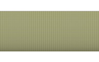
Meshing
Such channel flow analyses are usually conducted in two-dimensions when RANS (Reynolds Averaged Navier-Stokes)
turbulence models are used. DNS (Direct Numerical Simulation), LES (Large-Eddy Simulation) and hybrid models
do require a three dimensional domain and the numerical mesh.
The accuracy of the numerical approximation very much depends on the grid spacing near the wall. It is important
that the first few layers of the numerical grid reside inside the viscosity and thermal diffusivity dominated sublayer,
where the velocity (`u`) and the temperature (`theta`) profile exhibit the largest gradients.
Section of the hexahedral numerical grid near the wall for `Re_tau = 180` and `Pr = 0.71`
In all simulated cases, the numerical grid consists of hexahedral grid elements
elongated in the streamwise direction. The following grid resolutions are used with a different first grid layer spacing
(`Delta y_1`), and number of nodes (`n_y`) in the y-direction :
`y_1^+ = 0.5`, which leads to
`Delta y_1 = 0.278` `"mm"` and `n_y = 93` for `Re_tau = 180` and `Pr = 0.71`
`Delta y_1 = 0.127` `"mm"` and `n_y = 203` for `Re_tau = 395` and `Pr = 0.71`
`y_1^+ = 0.5//Pr`, which leads to
`Delta y_1 = 0.0556` `"mm"` and `n_y = 460` for `Re_tau = 180` and `Pr = 5.0`
The grid spacing is uniform in the streamwise (x) direction with 128 grid elements. Due to two-dimensionality
of the mean velocity (`bar(u)`) and the temperature (`bar(theta)`) field, only few grid elements (i.e. 8) are used across the domain in
the z-direction.
Initial conditions
Steady-state problem, initial conditions can be arbitrary.
Boundary conditions
In the streamwise (x) direction, the momentum and thermal boundary conditions are periodic.
At the bottom surface, no-slip boundary condition `u = 0.0 "m"//"s"` shall be
prescribed. A fixed temperature `theta = 0.0` `"K"` is used as a boundary condition
for the linearised energy transport equation [3 & 4].
Only a half of the channel can be simulated by utilising symmetry boundary conditions
at the channel mid-plane (top boundary).
For the vertical X-Y surfaces, the symmetry or equivalent conditions shall be used.
Results
Steady-state simulations were performed using the Shear Stress transport (SST) turbulence model in a double precision CFD solver.
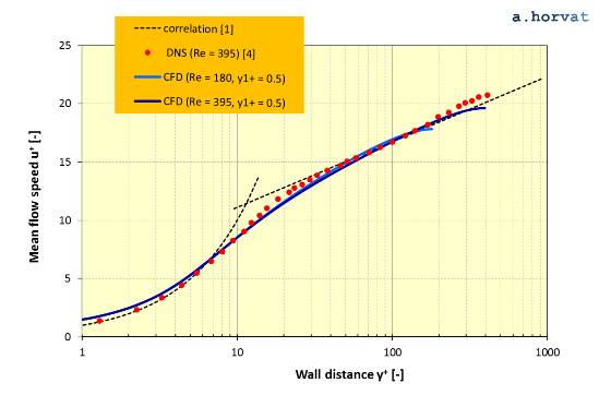
The cross-channel profile of mean streamwise velocity (`bar(u)`) was extracted from the CFD
simulation results, and compared with the empirical correlation [1] and the DNS results of
Kawamura et al. [4] in the dimensionless form:
`y^+ = (rho u_tau y)/mu`; `u^+ = bar(u)/u_tau`; `u_tau = (mu Re_tau)/(rho delta)`
The near-wall velocity profiles shows the viscosity dominated sublayer, where the
velocity profile is linear:
`u^+ = y^+`
and the outer logarithmic region
`u^+ = 1/kappa ln(y^+ )+B`
where `kappa` is the von-Karman constant (0.41) and `B` is 5.2 [1].
Near-wall mean velocity (`u^+`) profile in turbulent channel flow
For validation purposes, quadratic mean (or RMS) of deviation between the DNS data [4] and
the CFD simulation results is calculated for `Re_tau = 395`:
Reynolds number (`Re_tau`)
RMS of deviation
`y_1^+ = 0.5`
395
0.43
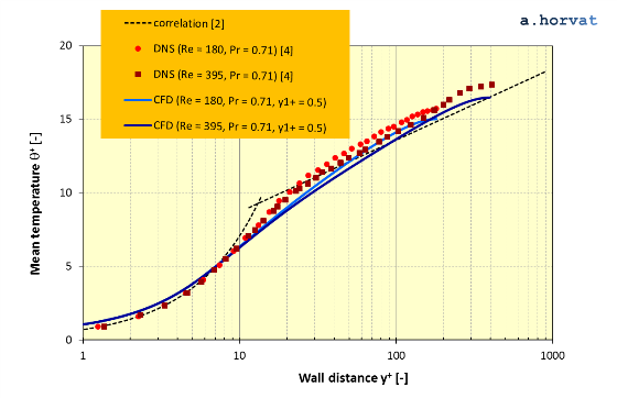
The cross-channel profile of mean temperature (`bar(theta)`) shall be obtained from the CFD results,
and compared to the empirical data [2] and the DNS results [3 & 4] in the dimensionless form:
`theta^+ = bar(theta)/theta_tau`; `theta_tau=q_w/(rho c_p u_tau )`
Similar to the viscosity dominated momentum sublayer, a thermal sublayer is formed near the wall.
Its thickness is related to the momentum sublayer by Prandtl number:
`y_(th)^+= y^+Pr`
The empirical correlations approximate the temperature profile (`theta^+`) in two regions - the linear
distribution close to the wall:
`theta^+ = y^+ Pr`
and the logarithmic profile in the outer region [2]:
`theta^+ = 2.12 ln(y^+ Pr) + (3.85 Pr^(1//3)-1.3)^2`
The temperature profile near the wall is affected by thermal diffusivity as well as by the flow velocity
distribution. When the Prandtl number departs significantly from value of 1.0, more complex empirical
relations are used for the region between the linear and the logarithmic profile [2].
Near-wall mean temperature (`theta^+`) profile in turbulent channel flow at Pr = 0.71
Quadratic mean (or RMS) of deviation between the DNS data [3 & 4] and the CFD simulation results is calculated
for `Re_tau = 180` and `395` (`Pr = 0.71`):
Reynolds number (`Re_tau`)
RMS of deviation
`y_1^+ = 0.5`
180
0.67
`y_1^+ = 0.5`
365
0.59
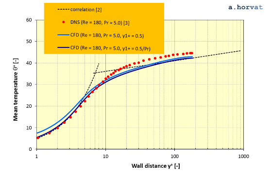
Near-wall mean temperature (`theta^+`) profile in turbulent channel flow at Pr = 5.0
Quadratic mean (or RMS) of deviation between the DNS data [3] and the CFD simulation results is calculated
for `Re_tau = 180` (`Pr = 5.0`):
Reynolds number (`Re_tau`)
RMS of deviation
`y_1^+ = 0.5`
180
2.04
`y_1^+ = 0.5//Pr`
180
2.17
The accuracy of the results depends fundamentally on the grid resolution in the near-wall sublayer, where viscous forces and
diffusive heat fluxes are dominant. For that reason, comparing accuracy of different numerical algorithms shall only be conducted when
the simulation results were obtained with a numerical grid of the same near-wall resolution.
S. B. Pope, Turbulent flows: 7.1.4. Mean velocity profiles, 2000, Cambridge University Press, p. 274.
B. A. Kader, Temperature and concentration profiles in fully turbulent boundary layers. Int. J. Heat Mass transfer, 1981, 24, pp. 1541-1544.
H. Kawamura, K. Ohsaka, H. Abe, K. Yamamoto, DNS of turbulent heat transfer in channel with low to medium-high Prandtl number, Int. J. Heat Fluid Flow, 1998, 19, pp. 482-491.
H. Kawamura, H. Abe, Y. Matsuo, DNS of turbulent heat transfer in channel with respect to Reynolds and Prandtl number effects, Int. J. Heat Fluid Flow, 1999, 20, pp. 196-207.
Dr Andrei Horvat
M.Sc. Mechanical Eng.
Ph.D. Nuclear Eng.