Introduction
Kelvin-Helmholtz instability is one of basic cases of flow instability. It is responsible for a wide range of phenomena in the natural environment (e.g. ocean waves, atmospheric flows) and in industrial installations (e.g. slug formation, water hammer).
The Kelvin-Helmholtz instability develops at the interface between two fluids that are moving at different velocities. Small interface deformations influence the local pressure distribution, which may amplify the initial deformations. Shear forces between both fluid streams distort the initially linear waves into a much more complex interface topology.
Although, the problem of Kelvin-Helmholtz instability is theoretically well defined [1], the experimental studies suitable for CFD validation purposes are rare. The present validation case is based on the theoretical and experimental work of Thorpe [2].

Objectives
The two-fluid laminar flow case examines the interaction between the flow field development (pressure and velocity) and the interface deformation (wave number and amplitude). Transient CFD simulations shall be used to compare (a) the most unstable wave number, (b) the time of onset of the instability, and (c) the instability growth rate with the theoretical and experimental data.
In multiphase flows, the calculation of interface position is directly related to mass conservation of both fluids. Therefore, the largest errors are most likely associated with the mass transport equations, especially in absence of large density gradients. Different numerical models may be implemented to stabilize the convergence behaviour, although they may adversely affect the wave growth rate.

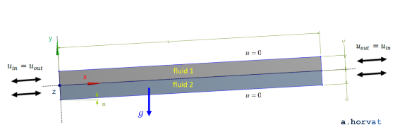
Geometry

• Length of the channel (L) is 1.83 m.
• Height of liquid layers (h = h₁ = h₂) is 0.015 m.
• Channel tilt angle (`alpha`) is 4.13°.
• Domain width is 0.1 m (although not important due to the case two-dimensionality).

A shorted channel can be used if flow periodicity between the inlet and the outlet is enforced.

Loading

• The fluid motion is induced by the tube inclination angle `alpha`.
• If the channel is simulated as a horizontal periodic section, appropriate momentum sources need to be assigned [3] in the horizontal direction:
`S_x = - rho g (rho/rho_(ave)-1)sin(alpha)`       where   `rho_(ave)=(rho_1+rho_2)//2`
• Gravity force also needs to be reduced to
`S_y = - rho g cos(alpha)`     where   `g=9.81` `"m"//"s"^2`

Material properties
Two fluids are used in the setup [2]. For the top layer, a mixture of carbon tetrachloride and commercial paraffin leads to the following properties:

• `rho_1` is density of 780 kg/m³
• `mu_1` is dynamic viscosity of 0.0015 Pa s

For the bottom layer, water material properties should be used:

• `rho_2` is density of 1000 kg/m³
• `mu_2` is dynamic viscosity of 0.001 Pa s

Surface tension `sigma` between both fluids is 0.04 N/m.

Meshing
In all simulated cases, the numerical grid consists of hexahedral grid elements that are compressed near the interface of both fluids.
In the vertical (y) direction, the grid spacing near the interface is 0.15 mm, which is then expanded to 0.30 mm near the bottom and the top boundary.

In the streamwise (x) direction, a uniform grid spacing of 0.15 mm is used, whereas in the z-direction, the 2D grid elements are extruded for a single grid spacing across the simulation domain.

Initial conditions

• Initially, both layers are at rest; therefore zero velocity conditions should be assigned.
• Random disturbances may be introduced to the two-fluid interface elevation at the start of the simulation to stimulate the development of the Kelvin-Helmholtz instability [4]. These elevation changes shall be much smaller than the near interface grid spacing.

Boundary conditions

• In the original experiment, the channel was closed. Therefore, no-slip boundary conditions can be applied at the bottom and the top wall.
• If the channel is modelled as a periodic section, periodicity of velocity components `(u_(i\n)=u_(out))` as well as volume fractions `(r_(i\n)=r_(out))` needs to be imposed at both ends in the streamwise (x) direction.
• For the vertical X-Y surfaces, the symmetry or equivalent conditions shall be used.

Results
Transient CFD simulations were performed using a laminar homogeneous multiphase model and a double precision solver.
In the first simulation, which did not include the surface tension force, the timestep was 0.001 s. The timestep was substantialy reduced to 0.0002 s in the second simulation, when the surface tension was incorporated in the model.

The volume fraction distribution calculated in each timestep is used to estimate time evolution of the most unstable wave number. For the current case, the theoretical critical wave number is close to its deep fluid limit:
`k_c=sqrt(g(rho_2-rho_1)//sigma)`
The measured value of the wave number at the onset of the Kelvin-Helmholtz instability [2 & 5] is
`k=(0.85+-0.25)k_c=197+-58` `"m"^(-1)`
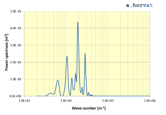
Although Fourier spectrum analysis can be employed to find the wave number with the largest amplitude, the most unstable wave number is usually estimated visually as a median of the dominant wave group. From the CFD results, the most unstable wave number is estimated to be approximately `188` `"m"^-1`.

Temporal development of the average wave amplitude is calculated from the CFD results to determine the onset of the Kelvin-Helmholtz instability and the growth of disturbances. The amplitude growth should then be calculated based on the amplitude of the initial disturbance in the model.
Thorpe [2] advises to use the time at which a disturbance grows to 100 times its initial amplitude as the onset of instability:

• the lowest theoretical time for the onset of instability is obtained from the linear stability theory [2] using `k=1.45k_c`  which gives  `t_(100(min))=1.52` `"s"`
• the experimentally observed time for the onset of instability is `1.79` `s<=t_(100(exp))<=1.92` `"s"`

Based on the CFD simulation results, the time to the onset of instability (`t_(100)`) is calculated to be `1.54` `s`, when the surface tension force is neglected. The time increases to `1.73` `s`, when the surface tension model is also included.
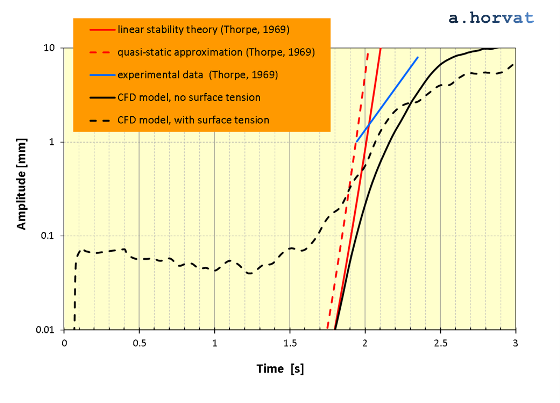
The wave amplitude growth can be calculated using the linear stability theory. It is expressed with the Airy function of the second kind [2]:
`N=(Bi(s))/(Bi(0))`
where

• `s=(-a)^(1//6)tau_1`,   `a = -((sigma k^2+(rho_2-rho_1) g cos(alpha)) h (rho_1+rho_2) tanh(kh))/(4g sin(alpha)(rho_2-rho_1) h sqrt(rho_1 rho_2))` ,
• `tau_1=tau-2 sqrt(-a)`,   `tau = t{(4 g sin(alpha) k (rho_2-rho_1) sqrt(rho_1 rho_2))/(rho_1+rho_2)^2}^(1//2)`.

Thorpe [2] also presents a quasi-static approximation of the wave amplitude growth that can be used for comparison:
`N=|eta(tau)|/|eta(0)|=(exp{tau/2 a^(1//2) (1-b^2)^(1//2)})/{b+[b^2-1]^(1//2)}^(-a)`     where   `b=tau/(2 sqrt(-a))`
The diagram below compares the wave amplitude (`eta`) that is calculated from the CFD simulation results with the linear stability theory and the quasi-static approximation [2]. The wave amplitude is defined as `sqrt(2) sigma`, where `sigma` is the standard deviation of the interface elevation across the simulation domain.

From the available experiment visualisation data, Thorpe [2] also estimates the wave growth factor (`beta`) to be 5.1 s^-1:
`(d|eta|)/dt = beta|eta|` Nevertheless, the assumption of constant wave growth is valid only for a very limited time interval between `1.2` `t_(100)` and `1.45` `t_(100)`. In this range, the wave is large enough to be visible and still unaffected by the presence of the horizontal tube walls.

Files

• Wave amplitude growth, analytical model [2] (2016/03/20)
• Wave amplitude, experimental data [2] (2016/03/20)