Introduction
Flow of an electrically conductive fluid across a magnetic field induces an electric current. The resulting Lorentz force may profundly affect the flow behaviour. Examples of such magneto-fluid dynamics occur in plasmas, liquid metals, molten salts and electrolytes.
Designing power systems or process equipment in which magneto-fluid dynamic effects are significant requires understanding of the flow and its development due to the imposed magnetic field.
In the examined cases, a two-dimensional flow layer is subjected to such transverse, external magnetic field. Due to low magnetic Reynolds number, the impact of the induced magnetic field can be neglected. A simplified arrangement, for which an analytical approximation exists, offers a suitable benchmark test for CFD modelling capabilities.

Objectives
In flow that is subjected to a transverse magnetic field, the volumetric Lorentz force may become a dominant factor shaping the flow field. As it acts in the opposite direction to the local flow velocity vector, it decelerates the flow motion and increases the associated pressure drop. Therefore, such magneto-fluid dynamic flow regime represents a significant challange to stability of CFD solvers.
Studied cases represent a very basic arrangement of the magneto-fluid dynamic regime, where a conductive fluid layer is subjected to an external magnetic field [1]. Three variations with different electric field boundary conditions are analysed in order to test the solver stability and its ability to find a numerical, steady-state solution.

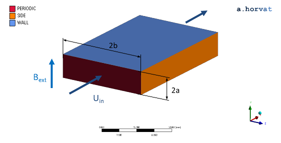
Geometry

• Height of the layer (2 a) is 0.01 m.
• Width of the layer (2 b) is 0.04 m.
• Length of the simulation domain is 0.06 m.

As the current density field is solenoidal, its two-dimensionality in the spanwise (z) direction can only be modelled by extending the width of the simulation domain (2 b).
The flow is periodic in the streamwise direction. Therefore, the length of the simulation domain can be selected with an aim to enhance convergence of the CFD simulation.
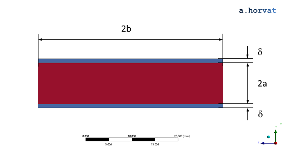
Where the electrically conductive bottom and top walls are included in the CFD model (i.e. in the conjugate cases), the simulation domain also contains the additional horizontal layers with the thickness (`delta`) of 0.001 m.

Loading
The fluid motion is induced by the prescribed pressure gradient in the streamwise (x) direction that corresponds to a selected Reynolds number (`Re`) value:
`u_0 = (mu Re)/(rho a) `     and     `(dp)/(dx) = - (mu u_0)/(a^2)`
where `u_0` is the velocity scale, `mu` is the fluid's dynamic viscosity and `rho` its density.
The magnetic field is defined by selected Hartmann number (`Ha`) values: `B = (Ha)/a sqrt(mu/sigma)`
where `mu` is the fluid's dynamic viscosity and `sigma` its electric conductivity.
Four groups of cases with an equal Reynolds number, but a different Hartmann number are used in the assessment. Their pressure drop (`dp//dx`) and magnetic field flux density (`B`) are: 1)   `Re = 2000`   &   `dp//dx =`-`1.625*10^-3` `"Pa"//"m"`,  `Ha = 0.0`   &   `B = 0.0` `"T"`
2)   `Re = 2000`   &   `dp//dx =`-`1.625*10^-3` `"Pa"//"m"`,  `Ha = 2.0`   &   `B = 0.761*10^-2` `"T"`
3)   `Re = 2000`   &   `dp//dx =`-`1.625*10^-3` `"Pa"//"m"`,  `Ha = 5.0`   &   `B = 1.901*10^-2` `"T"`
4)   `Re = 2000`   &   `dp//dx =`-`1.625*10^-3` `"Pa"//"m"`,  `Ha = 10.0`   &   `B = 3.803*10^-2` `"T"`

Material properties
The material properties of NaK eutectic [2 & 3] are used for the simulated cases:

• `Y_(K)`  is potassium mass fraction of 77.8 %
• `rho`  is density of 870 kg/kmol
• `mu`  is dynamic viscosity of 9.4·10^-4 Pa s
• `sigma`  is electrical conductivity of 2.6·10⁶ S/m

For the conjugate cases, material properties of 316 stainless steel [4] are selected for the solid layers:

• `sigma_s`  is electrical conductivity of 1.3·10⁶ S/m,

which yields the wall conductance `c = sigma_s delta//sigma a`  of 0.1.

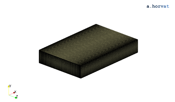
Meshing
In all simulated cases, the numerical grid consists of hexahedral grid elements:

• The uniform spacing of 0.001 m is applied in the streamwise (x) direction.
• In the horizontal (z) direction, 80 elements are employed with a bias factor (16) to refine the grid near both vertical boundaries.
• In the vertical (y) direction, 60 elements are used with a bias factor (20) to refine the grid near both horizontal surfaces.

The utilised numerical grid contains 0.301 mil nodes and 0.288 mil elements.

For the conjugate cases, 12 elements are employed in the vertical direction for each solid layer with a bias factor (6) to refine the grid near the interface with the fluid flow domain. This increases the number of grid nodes to 0.420 mil and the number of elements to 0.403 mil.

Initial conditions
Steady-state CFD simulations are used for comparison with the experimental data. Although their initial conditions can be arbitrary, they should enhance stability of the solution procedure.
For that purpose, it is advised to start with the CFD simulation of forced convection without the external magnetic field. When the flow field is fully developed, the external magnetic field is reintroduced.

Boundary conditions

• In the streamwise (x) direction, the momentum and electric field boundary conditions are periodic.
• At the bottom and the top surface, no-slip conditions `u = 0.0` `"m"//"s"` are prescribed. Three cases with different electric field boundary conditions are investigated:
  
  1)   non-conductive boundaries with electric current density `j = 0.0` `"A"//"m"^2`
  2)   infinitely conductive boundaries with electric potential set to `phi = 0.0` `"V"`
  3)   boundaries coupled to the solid domain with `j` preserved in the normal direction
  
  At the bottom and the top boundary of the solid domain (case 3), the non-conductive electric current conditions (`j = 0.0` `"A"//"m"^2`) are prescribed.
• At the vertical, side surfaces, the symmetry or equivalent conditions can be used for the fluid flow. The electric field requires the non-conductive boundary conditions (`j = 0.0` `"A"//"m"^2`) to enforce solenoidity of the electric current across the simulation domain.

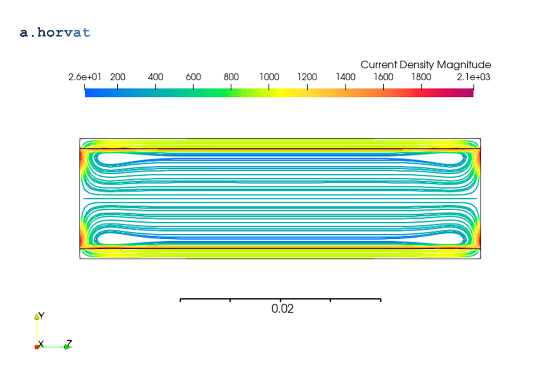
Results
Steady-state CFD simulations were conducted with a double precision CFD solver. The timescale 0.1 - 1.0 s was used to obtain converged results.

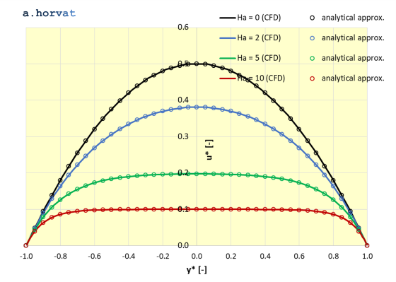
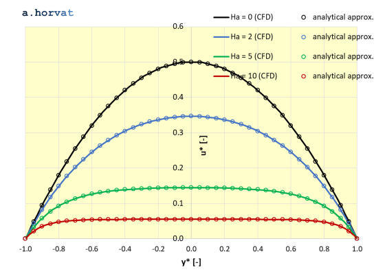
The CFD results are compared with an analytical, 2D approximation of the streamwise flow velocity [1] across the simulation domain. The velocity profile in the direction of the imposed magnetic field is expressed as:
`u^ star = hat u [1 - cosh (y^ star Ha)/cosh(Ha)]`
where `u^ star = u//u_0` is the dimensionless flow speed and `y^ star = y//a` the dimensionless vertical location. In addition, the characteristic magnitude of velocity is defined as:
`hat u = 1/(Ha)[(c+1)/(c Ha + tanh(Ha))]`
A parabolic velocity profile that corresponds to the forced convection flow in absense of a magnetic field (Ha = 0):
`u^ star = 0.5 [1 - (y^ star)^2]`
is added to comparison.
Non-conductive bottom and top boundary

For validation purposes, quadratic mean (or RMS) of deviation between the analytical approximation [1] and the CFD simulation results is calculated for the streamwise velocity (`u^ star`) along the centreline:

Hartmann number	RMS of deviation
0.0	7.05E-4
2.0	2.75E-4
5.0	1.41e-4
10.0	1.27e-4

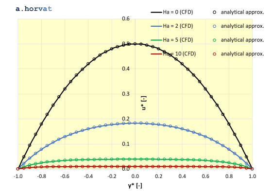
Infinitely conductive bottom and top boundary

For validation purposes, quadratic mean (or RMS) of deviation between the analytical approximation [1] and the CFD simulation results is calculated for the streamwise velocity (`u^ star`) along the centreline:

Hartmann number	RMS of deviation
0.0	7.05E-4
2.0	1.22E-4
5.0	1.41e-4
10.0	1.54e-6

Electrically coupled bottom and top boundary

For validation purposes, quadratic mean (or RMS) of deviation between the analytical approximation [1] and the CFD simulation results is calculated for the streamwise velocity (`u^ star`) along the centreline:

Hartmann number	RMS of deviation
0.0	7.05E-4
2.0	2.31E-4
5.0	6.45e-5
10.0	3.66e-5

Files

• Streamwise velocity - analytical results for non-conductive boundaries (2023/01/14)
• Streamwise velocity - infinitely conductive boundaries (2023/01/14)
• Streamwise velocity - electrically coupled boundaries (2023/01/14)