... from an idea to superior design performance with mathematical modelling and engineering analysis ...
Channel flow with viscous heating
Introduction
Channel flow is one of basic flow arrangements that can be found in many
engineering systems. In processes with highly viscous working fluids, shear may
contribute importantly to the overall energy balance. Such viscous heating that
is often characterised by Brinkman number has to be taken into account
in polymer processing as well as in food process industry.
Thermally developing Poiseuille flow case has also an educational value.
It is a mathematically well-defined problem and for which an analytical solution
exists. For that reason, it is an integral part of many graduate courses in
fluid mechanics.
Objectives
The case may represent a validation challenge as the momentum dissipation serves
as a significant source of thermal energy. Although, the flow velocity profile
is fully developed and steady, the imposed thermal boundary conditions cause
a very pronounced thermal entrance effect.
The model validation is based on a comparison of the simulated temperature profiles
between two parallel plates with the analytical solution of the extended
Graetz-Nusselt problem [1]. In addition, the flow mean temperature and the wall
Nusselt number distribution along the channel wall are also used for the comparison.
Any effects of numerical diffusion will lower the temperature profile. Also,
large diffusion constants (i.e. kinematic viscosity and thermal diffusivity) may
impose stability restrictions on the size of the timestep used in the explicit CFD codes.
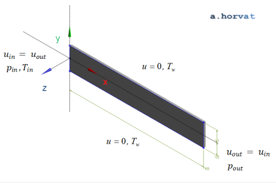
Geometry
Total length of the channel (H3) is 0.8 m.
Channel half-width (V1 = V2) is 10.0 mm.
Height is 1.0 mm (although not important due to the case two-dimensionality).
Loading
Four cases with a different pressure drop across the domain are investigated:
`Delta p//L_x =" - "4.0," - "40.0, " - "400.0`
and `" - "4000.0" kPa/m"`.
The imposed pressure drop results in a fully developed flow with the maximum velocity
`u_max = 0.02, 0.2, 2.0` and `20.0" m/s"`.
The inlet temperature (`T_(\i\n)`) is set above the wall temperature (`T_w`), which cools the flow.
It is the viscous heating associated with the fluid velocity gradient that raises the temperature in the flow.
Material properties
The following fluid material properties that correspond to polymer processing are used for all investigated cases:
`rho` is density of 500.0 kg/m3;
`mu` is dynamic viscosity of 10.0 Pa s;
`c_p` is specific heat capacity of 1000.0 J/kgK;
`lambda` is thermal conductivity of 1.0 W/mK.
The Prandtl number (`Pr= c_p` `mu//lambda`) is 10,000 in all cases.
Meshing
In all simulated cases, the numerical grid consists of hexahedral grid elements
elongated in the streamwise direction. The uniform spacing of 0.002 m is used
in the x-direction. In the perpendicular direction, the numerical mesh
is significantly refined near the wall to 0.00008 m.
In the z-direction, the 2D grid elements are extruded for a single grid spacing
across the simulation domain.
Section of the hexahedral numerical grid refined near the wall
Initial conditions
The solution of such extended Graetz-Nusselt problem can be simplified since
the solution of the fully developed velocity field is known in advance.
In such case, the parabolic velocity profile and zero pressure can be prescribed at
the start of the simulation:
`u=-(b^2)/(2 mu )((Delta p)/L_x) (1-y^2/b^2 )` where `b` is
the channel half-width.
Boundary conditions
As the velocity field is known in advance, the solution of the momentum equation
is not required. For that reason, only the energy equation boundary conditions
are prescribed:
At the inlet boundary `T_(\i\n)=30^"o""C"`.
At the top and bottom wall, the reduced temperature `T_w = 20^"o""C"` is assigned.
For the vertical X-Y surfaces, the symmetry or equivalent conditions shall be used.
Results
The effect of thermal conduction in the axial direction can be neglected for large Peclet
numbers (Pe `>=` 100), which leads to the following simplified differential equation:
`(1-eta^2) del_(xi) hat T = del_eta del_eta hat T + 4 eta^2 Br`, `hat T(0,eta)=1` and `hat T(xi,-1)=hat T(xi,1)=0`
where
`eta=y//b`, `xi=x//bPe`, `hat u=u//u_(max)`, `u_(max)=`-`Delta p b^2//2 mu L_x`,
`hat T =(T-T_w)//Delta T`, `Delta T=T_(\i\n)-T_w`,
`Pe=RePr`, `Re=rho u_(max) b//mu`, `Pr=c_p mu//lambda`, `Br=mu u_(max)^2//lambda Delta T`.
The exact solution of the non-homogeneous differential equation can be found in the form of:
`hat T = sum_(k=1)^m C_k exp( " - "beta_k xi ) sum_(i=1)^n A_(ki) cos( (i-1//2) pi eta) + 1/3 Br (1 - eta^4)`
The eigenvalues (`beta_k`) and the coefficients of the series (`C_k`) can be
downloaded in the file section below.
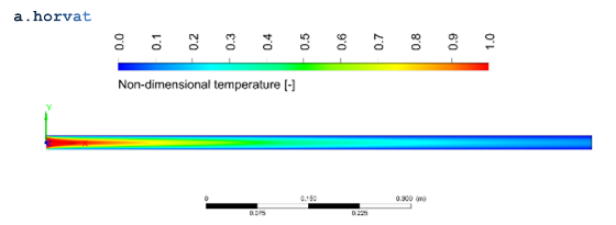
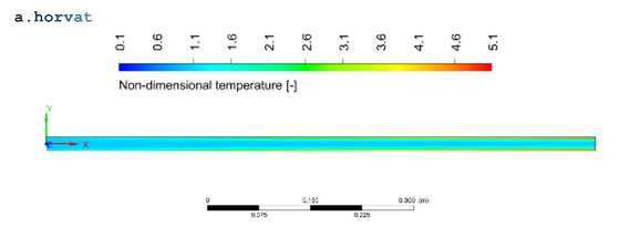
Distribution of dimensionless temperature (`hat T`) in the channel at Br = 0.0004
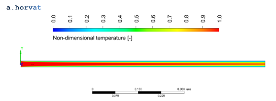
Distribution of dimensionless temperature (`hat T`) in the channel at Br = 0.04
Distribution of dimensionless temperature (`hat T`) in the channel at Br = 4.0
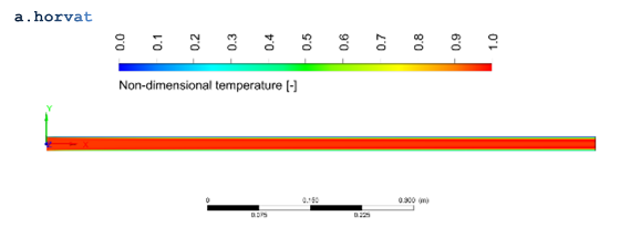
Distribution of dimensionless temperature (`hat T`) in the channel at Br = 400.0
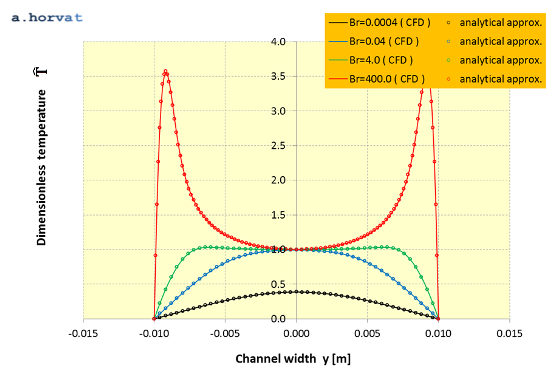
Steady-state simulations were performed using a single precision CFD solver.
For validation purposes, the dimensionless temperature profile `hat T(y)`
across the channel is calculated at x = 0.4 m. Four cases with a different
imposed pressure drop lead to a different value of Brinkman number (i.e. 0.0004,
0.04, 4.0 and 400.0), which impacts thermal conditions. The obtained profiles
are compared with the analytically derived values.
Quadratic mean (or RMS) of deviation between the analytical solution and
the CFD simulation results for the dimensionless temperature vertical
profile at x = 0.4 m is:
Brinkman number
RMS of deviation
0.0004
4.63E-3
0.04
6.93E-5
4.0
2.41e-4
400.0
1.62e-3
Dimensionless temperature profile (`hat T`) at x = 0.4 m for different values of Brinkman number
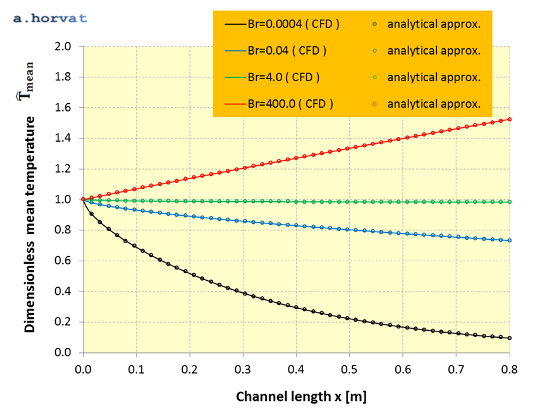
The flow mean temperature is defined as
`T_(mean) = 1/(u_(mean) 2b) int_(-b)^b uT dy`
Its dimensionless form `hat T_(mean) = (T_(mean)-T_w )//Delta T` is calculated
from the CFD results and compared with analytical values along the channel.
Quadratic mean (or RMS) of deviation between the analytical solution and the
CFD simulation results for the dimensionless mean temperature along the channel is:
Brinkman number
RMS of deviation
0.0004
1.06E-3
0.04
3.29E-4
4.0
1.43e-4
400.0
8.08e-4
Dimensionless mean temperature (`hat T_(mean)`) along the channel for different values of Brinkman number
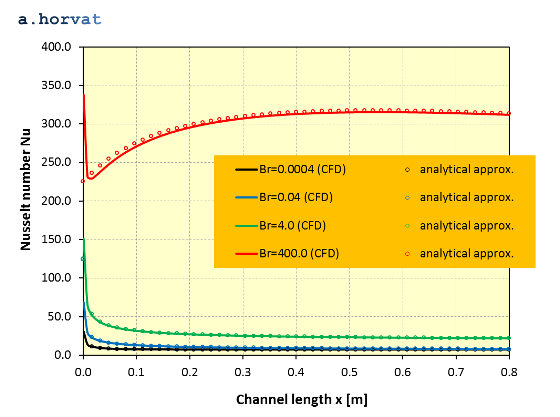
Nusselt number along the channel is defined as
`Nu=(q_w" "4b)/(k(T_w-T_(mean) ))`
The calculated Nusselt number are compared with the analytically obtained values. Quadratic mean (or RMS)
of deviation between the analytical solution and the CFD simulation results for Nusselt number along the channel is:
R.K. Shah and A.L. London, Laminar flow forced convection in ducts:
A source book for compact heat exchanger analytical data: Laminar flow forced
convection in ducts, Academic Press, 1978, p. 170.
H. Schlichting, Boundary layer theory, McGraw-Hill, 7th Ed, 1979, p. 281.
Dr Andrei Horvat
M.Sc. Mechanical Eng.
Ph.D. Nuclear Eng.