Introduction
Flows arising from thermal buoyancy are frequently encountered in many environmental and man-made systems. In most cases buoyant flows are highly turbulent and often unstable. Moreover, far from the buoyancy source relaminarisation of turbulent flow can also occur. Such complex nature of buoyant flows makes their modelling still a very demanding task.
The assessed cases examine free shear flow behaviour, where the flow is induced by imposing momentum and/or heat flux in absence of wall effects. The role of buoyancy, which is characterised by Richardson number, is examined by increasing its value from 0.0 (i.e. force convection flow) to 1.0.

Objectives
In force convection and buoyancy induced jets, the flow acceleration causes pressure to decrease, and consequently to entrainment the surrounding fluid. In addition, correct modelling approximation of turbulence production and decay is required.
The validation cases test the ability of the implemented turbulence model to predict flow conditions in force convection and in buoyancy driven, free shear flow scenarios. For that purpose, calculated axial and radial distributions of flow velocity and temperature shall be compared to experimental values [1-4] in order to expose any modelling deficiencies and numerical errors (e.g. discretisation mistake, false numerical diffusion, equation under-relaxation).

Geometry

• Diameter of the supply pipe (d) is 0.24 m.
• Length of the supply pipe ( l = 20 d) is 4.8 m.
• Diameter of the simulation domain (D_amb = 40 d) is 9.6 m.
• Length of the simulation domain (L_amb = 120 d) is 28.8 m.

Using axisymmetry, the simulation domain can be a two-dimensional tangential slice of the annular geometry. Poor convergence due to restrained entrainment may force the user to simulate a wider tangential section.
For Large-Eddy Simulation (LES) or Direct Numerical Simulation (DNS) modelling, a full 360° simulation domain is required.

Loading
The fluid motion is induced by the prescribed specific momentum (`F_u`) and buoyancy (`F_b`) flux:
`F_u = 2 pi int_0^(d//2) u^2 r\dr`     and     `F_b = 2 pi int_0^(d//2) ub r\dr`
where `u` is the flow axial speed, and `b = g(rho_(amb) - rho)//rho_(amb)` is the specific weight deficiency.
Four cases with equal Reynolds number, but different Richardson number are used in the assessment. Their specific momentum (`F_u`) and buoyancy (`F_b`) flux are: 1)   `Re = 5000` & `F_u = 4.336*10^-3`,  `Ri = 0.0` & `F_b = 0.0`
2)   `Re = 5000` & `F_u = 4.336*10^-3`,  `Ri = 1.0` & `F_b = 5.401*10^-3`
3)   `Re = 5000` & `F_u = 4.336*10^-3`,  `Ri = 0.2` & `F_b = 1.115*10^-3`
4)   `Re = 5000` & `F_u = 4.336*10^-3`,  `Ri = 0.04` & `F_b = 2.245*10^-4`

Material properties
The ideal gas properties of air are used for the simulated cases:

• `M` is molar mass of 28.96 kg/kmol;
• `c_p` is specific heat capacity of 1004.4 J/kg K;
• `mu` is dynamic viscosity of 1.7894·10^-5 Pa s;
• `lambda` is thermal conductivity of 2.61·10^-2 W/mK.

Meshing
Hexahedral grid elements are used in all simulated cases.

• In the radial direction, the grid spacing in the supply pipe is 0.008 m, which is further decreased near the wall to 0.0024 m. Away from the wall towards the external boundary, the grid spacing expands again to 0.092 m.
• In the tangential direction, a uniform angular grid spacing of 4° is applied.
• In the axial direction, the grid spacing expands from 0.003 m near the orifice of the supply pipe, to 0.09 m downstream the jet in the far end of the simulation domain.

The utilised numerical grid contains 1.06 mil nodes and 1.05 mil elements.

Initial conditions
Steady-state CFD simulations utilising RANS turbulence modelling are used for comparison with the experimental data. Although their initial conditions can be arbitrary, they should enhance stability of the solution procedure.
For visualisation purposes, transient LES modelling is used. For such purpose, the initial conditions in the simulation domain are equal to the ambient conditions (`p_(amb)` & `T_(amb)`) and zero flow speed.

Boundary conditions

• The pipe inflow boundary conditions for examined cases are:
  
  1)   `Ri = 0.0`, `u_(i\n) = 0.3096` `"m"//"s"`, `T_(i\n) = 20.0^"o""C"`
  2)   `Ri = 1.0`, `u_(i\n) = 0.3096` `"m"//"s"`, `T_(i\n) = 32.0^"o""C"`
  3)   `Ri = 0.2`, `u_(i\n) = 0.3096` `"m"//"s"`, `T_(i\n) = 22.4^"o""C"`
  4)   `Ri = 0.04`, `u_(i\n) = 0.3096` `"m"//"s"`, `T_(i\n) = 20.48^"o""C"`
  
  In all cases, the turbulence intensity of the inflow is set to 5% and its eddy viscosity to `10mu`. The turbulence inflow conditions may be of secondary importance as long as the pipe flow is fully developed at its orifice.
• For the far-field boundary, opening boundary conditions are used that allow outflow as well as inflow due to local pressure conditions. The ambient pressure (`p_(amb)`) is set to 1.0 atm, and the local ambient temperature (`T_(amb)`) to 20.0°C.
  
  For the turbulence related transport variables (e.g. `k` and `epsilon`), zero gradient conditions are applied.
• No-slip, adiabatic boundary conditions are applied at the inner and the outer wall of the supply pipe.

Results
For visualisation of the flow field, LES modelling of the buoyant jet was conducted with a single precision CFD solver. A timestep of 0.004 s was used to simulate an overall time period of 30 s.

Force convection (Ri = 0.0)
For the comparison with the experimental data [1-4], steady-state CFD simulations were conducted using the `k`-`epsilon` turbulence model and a double precision CFD solver.
Following the work of List [1] and Hussein et al. [2], it is expected that the streamwise velocity (`u`) of the forced convection jet behaves in a self-similar region (`x` > 30d) as
`u \propto F_u^(1//2)x^(-1)f(r)`
where the function `f(r)` represents jet's radial behaviour and it acquires a constant form in the self-similar region. For the streamwise velocity along the centreline (`u_c`), the following correlations published by List [1]:
`u_c(d^2/F_u)^(1//2) = 7.0 (x/d)^(-1)`
and by Hussein et al. [2]:
`u_c(d^2/F_u)^(1//2) = 6.7 (x/d)^(-1)`
are used for comparison with the CFD simulation results.

Using the same scaling, a radial profile of the streamwise flow velocity (`u_c`) is calculated and compared with the correlation presented by List [1]:
`u(x^2/F_u)^(1//2) = 7.0 exp( -alpha_u(r/(beta_u x))^2 )`     where `alpha_u = 1.0` & `beta_u = 0.107`
and by Hussein et al. [2]:
`u(x^2/F_u)^(1//2) = 6.7 exp( -alpha_u(r/(beta_u x))^2 )`     where `alpha_u = 0.693` & `beta_u = 0.094`

For validation purposes, quadratic mean (or RMS) of deviation between the published correlations and the CFD simulation results is calculated for the streamwise velocity (`u`):

	RMS of deviation [1]	RMS of deviation [2]
streamwise velocity @ centreline `u_c(d^2//F_u)^(1//2)`	1.441e-2 (10 ≤ `x//d` ≤ 100)	6.236e-3 (10 ≤ `x//d` ≤ 100)
streamwise velocity @ `x//d` = 10 `u(x^2//F_u)^(1//2)`	4.108e-1 (0.0 ≤ `r//x` ≤ 0.25)	3.078e-1 (0.0 ≤ `r//x` ≤ 0.25)
streamwise velocity @ `x//d` = 20 `u(x^2//F_u)^(1//2)`	4.700e-1 (0.0 ≤ `r//x` ≤ 0.25)	3.432e-1 (0.0 ≤ `r//x` ≤ 0.25)
streamwise velocity @ `x//d` = 40 `u(x^2//F_u)^(1//2)`	4.948e-1 (0.0 ≤ `r//x` ≤ 0.25)	3.620e-1 (0.0 ≤ `r//x` ≤ 0.25)

Mixed convection (Ri > 0)
Simulation of buoyant flows does require modifications of the `k`-`epsilon` turbulence model coefficients [5-6]. Therefore, for all test cases where Ri > 0:
1) turbulence production term due to buoyancy was included only in the `k` transport equation,
2) eddy viscosity coefficient `C_(mu)` was increased from 0.09 to 0.18,
3) turbulent Prandtl number was set to 0.85.
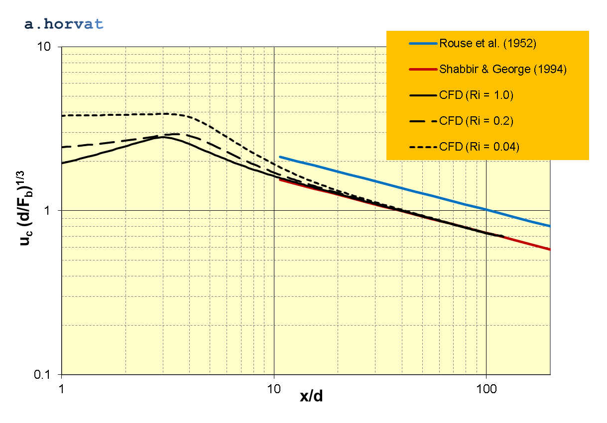
As discussed by Rouse et al. [3] and Shabbir & George [4], the streamwise velocity (`u`) of a buoyant jet complies in the self-similar region (`x` > 30d) with
`u \propto F_b^(1//3)x^(-1//3)f(r)`
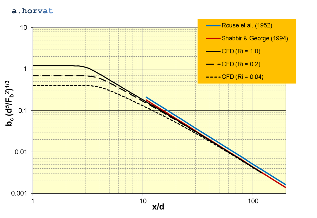
and the specific weight deficiency (`b`) with
`b \propto F_b^(2//3)x^(-5//3)f(r)`
Again, the function `f(r)` represents jet's radial behaviour and acquires a constant form in the self-similar region. For the streamwise velocity along the centreline (`u_c`) and the specific weight deficiency (`b_c`), the following correlations were published by Rouse et al. [3]:
`u_c(d/F_b)^(1//3) = 4.6 (x/d)^(-1//3)`
`b_c(d^5/F_b^2)^(1//3) = 11.0 (x/d)^(-5//3)`
Shabbir & George [4] later corrected their results to:
`u_c(d/F_b)^(1//3) = 3.4 (x/d)^(-1//3)`
`b_c(d^5/F_b^2)^(1//3) = 9.4 (x/d)^(-5//3)`

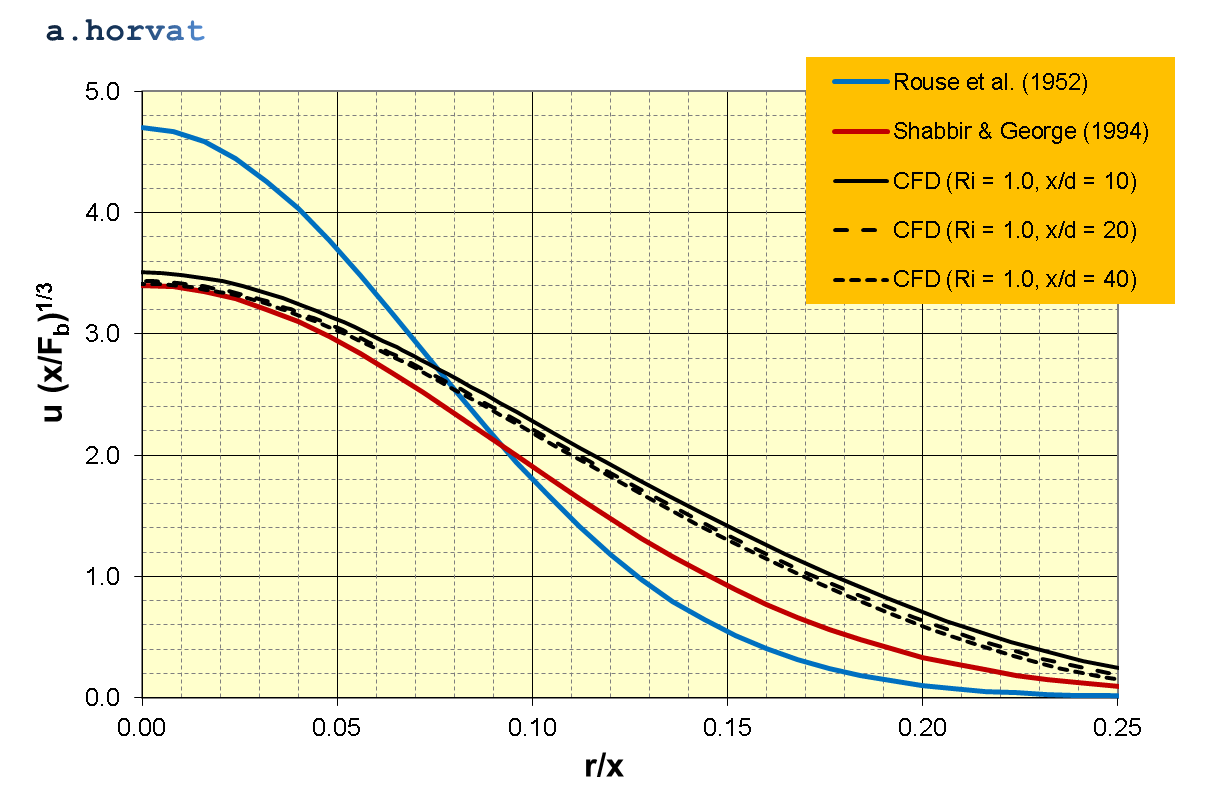
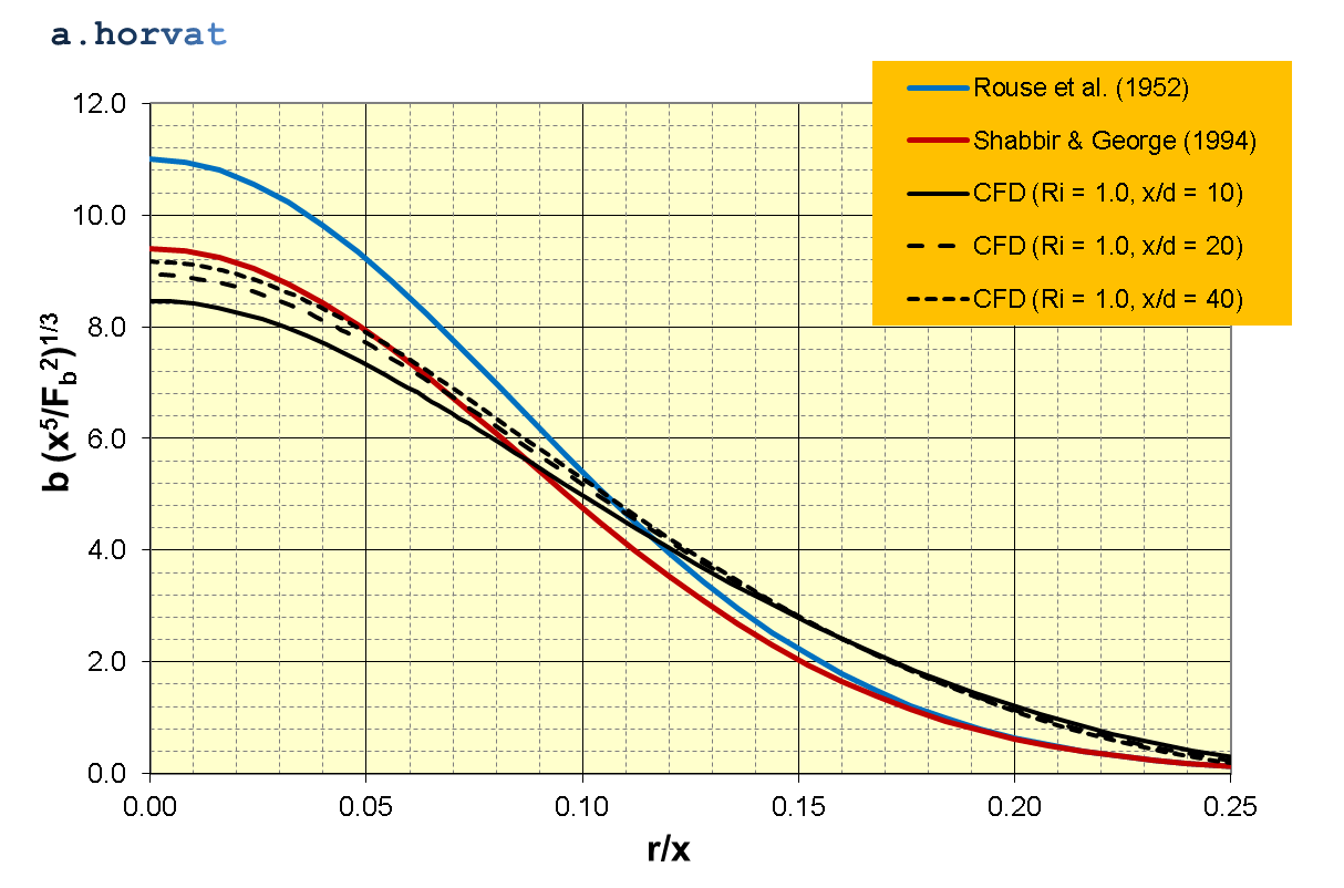
Radial profiles of the streamwise flow velocity (`u`) and the specific weight deficiency (`b`) are calculated only for the case with Ri = 1.0 and then compared with the correlations presented by Rouse et al. [3]:
`u(x/F_b)^(1//3) = 4.7 exp( -alpha_b(r/x)^2 )`      where `alpha_b = 96.0`
`b(x^5/F_b^2)^(1//3) = 11.0 exp( -alpha_b(r/x)^2 )`     where `alpha_b = 71.0`
and by Shabbir & George [4]:
`u(x/F_b)^(1//3) = 3.4 exp( -alpha_b(r/x)^2 )`     where `alpha_b = 58.0`
`b(x^5/F_b^2)^(1//3) = 9.4 exp( -alpha_b(r/x)^2 )`     where `alpha_b = 68.0`

For validation purposes, quadratic mean (or RMS) of deviation between the published correlations and the CFD simulation results is calculated for the streamwise velocity (`u`):

	RMS of deviation [3]	RMS of deviation [4]
streamwise velocity @ centreline `u_c(d//F_b)^(1//3)`	3.206e-1 (20 ≤ `x//d` ≤ 100)	4.179e-3 (20 ≤ `x//d` ≤ 100)
streamwise velocity @ `x//d` = 10 `u(x//F_b)^(1//3)`	6.697e-1 (0.0 ≤ `r//x` ≤ 0.25)	3.349e-1 (0.0 ≤ `r//x` ≤ 0.25)
streamwise velocity @ `x//d` = 20 `u(x//F_b)^(1//3)`	6.715e-1 (0.0 ≤ `r//x` ≤ 0.25)	2.762e-1 (0.0 ≤ `r//x` ≤ 0.25)
streamwise velocity @ `x//d` = 40 `u(x//F_b)^(1//3)`	6.604e-1 (0.0 ≤ `r//x` ≤ 0.25)	2.399e-1 (0.0 ≤ `r//x` ≤ 0.25)

and for the specific weight deficiency (`b`):

	RMS of deviation [3]	RMS of deviation [4]
sp. weight deficiency @ centreline `b_c(d^5//F_b^2)^(1//3)`	4.226e-3 (20 ≤ `x//d` ≤ 100)	7.571e-4 (20 ≤ `x//d` ≤ 100)
sp. weight deficiency @ `x//d` = 10 `b(x^5//F_b^2)^(1//3)`	1.163e+0 (0.0 ≤ `r//x` ≤ 0.25)	5.702e-1 (0.0 ≤ `r//x` ≤ 0.25)
sp. weight deficiency @ `x//d` = 20 `b(x^5//F_b^2)^(1//3)`	9.839e-1 (0.0 ≤ `r//x` ≤ 0.25)	4.907e-1 (0.0 ≤ `r//x` ≤ 0.25)
sp. weight deficiency @ `x//d` = 40 `b(x^5//F_b^2)^(1//3)`	8.811e-1 (0.0 ≤ `r//x` ≤ 0.25)	4.748e-1 (0.0 ≤ `r//x` ≤ 0.25)

Files

• Vertical distributions - correlation data [1 - 4]  (2019/03/24)
• Radial distributions - correlation data [1 - 4]  (2019/03/24)
• CFD simulation results for a force convection jet (Ri = 0.0) (2019/03/24)
• CFD simulation results for a buoyant jet (Ri = 1.0) (2019/03/24)
• CFD simulation results for a buoyant jet (Ri = 0.2) (2019/03/24)
• CFD simulation results for a buoyant jet (Ri = 0.04) (2019/03/24)